Why does the brain respond differently to the same sensory input from one moment to the next?
Neural responses are variable even when the outside world is held constant. Some of that variation reflects the stimulus itself. Some follows what an animal is doing. Some emerges from ongoing internal brain dynamics. These influences do not arrive in fixed proportions—and treating them as if they do can hide an essential feature of sensory processing: the neural code changes with state.
In our Nature Communications paper, “Deciphering Neuronal Variability Across States Reveals Dynamic Sensory Encoding”, led by my postdoc Shailaja Akella, we asked how the sources of visual-cortical variability reorganize over time.
In brief: The mouse visual cortex moved among three recurring oscillation states on a timescale of seconds. Each state had its own profile of neural variability and its own balance of stimulus, behavior, and internal brain influences. The high-frequency state, which was associated with greater arousal, supported the strongest representation of the visual stimulus, while the low-frequency state was more strongly shaped by internal dynamics.
Variability is part of the computation
It is tempting to treat response variability as noise—an unwanted deviation from a neuron’s “true” response. But variability has many possible sources, and those sources have different implications.
A neuron may vary because the visual scene is changing. Its activity may follow running, pupil dilation, or subtle facial and body movements. It may also reflect ongoing activity within its own area or signals arriving from elsewhere in the cortex. Even the same numerical amount of variability can therefore mean very different things.
The central challenge is time. Most encoding models learn one average relationship between these factors and neural activity. That approach is useful, but it assumes that their relative influence remains stable. The awake brain is not stationary: arousal fluctuates, behavior changes, and network activity moves among different regimes, often within seconds.
We wanted to preserve that temporal structure rather than average it away.
Finding a temporal backbone in brain activity
We analyzed the Allen Brain Observatory Visual Coding dataset: simultaneous Neuropixels recordings of spiking activity and local field potentials (LFPs) from six mouse visual cortical areas. The dataset included 25 awake mice passively viewing repeated presentations of a 30-second natural movie.
To identify internal states without defining them from behavior alone, we fitted a hidden Markov model to LFP signals spanning theta, beta, and low- and high-gamma frequency ranges across cortical areas and layers.
The analysis consistently revealed three oscillation states:
- a high-frequency state, dominated by gamma-range activity;
- an intermediate state; and
- a low-frequency state, dominated by slower theta-range activity.
These states were metastable: mice remained in one state for about 1.5 seconds on average before transitioning. Direct transitions between the low- and high-frequency states were uncommon; the brain generally passed through the intermediate state.
The states were strongly related to arousal and movement, but they were not interchangeable with a single behavioral measure. The high-frequency state coincided with larger pupils and more movement, whereas mice were usually quieter in the low-frequency state. Pupil size and facial movement tracked the inferred states more closely than running speed did. This distinction matters: internal brain state cannot be reduced to whether the animal is running.
Different states, different forms of variability
Neuronal variability is not one quantity, so we examined it in three complementary ways:
- shared variability—the fraction of variation coordinated across a neural population;
- trial-to-trial variability—how much spike counts differ across repeated presentations; and
- spike-timing variability—how irregularly spikes occur within a response.
The high-frequency state combined lower shared variability and lower trial-to-trial variability with greater spike-timing variability. At first glance, that last result may sound contradictory. In this experiment, however, irregular spike timing could reflect a more faithful response to the continually changing temporal structure of the natural movie rather than less reliable encoding.
Consistent with that interpretation, population activity in the high-frequency state carried more information about the movie frames than activity in the lower-frequency states. V1 retained the most pixel-level stimulus information. With the rostrolateral area as a notable exception, that information generally declined higher in the visual hierarchy.
The lesson is not that variability simply rises or falls with arousal. Its form changes. A state can reduce variability across trials while increasing temporally structured variation within a trial.
Separating stimulus, behavior, and internal dynamics
We next built a state-conditioned encoding model to ask what was driving neural activity in each state.
The model grouped predictors into three broad sources:
- visual stimulus features, including intensity, contrast, edges, energy, entropy, and kurtosis;
- behavior, including running and facial and body movements; and
- internal brain activity, represented by LFPs within the target area and average population activity in neighboring visual areas.
Separate regressors were learned within each oscillation state, allowing the model to follow changes in source contributions over time. Across the full dataset, it explained about 27% of single-neuron variability and 53% of the variance in area-averaged population activity.
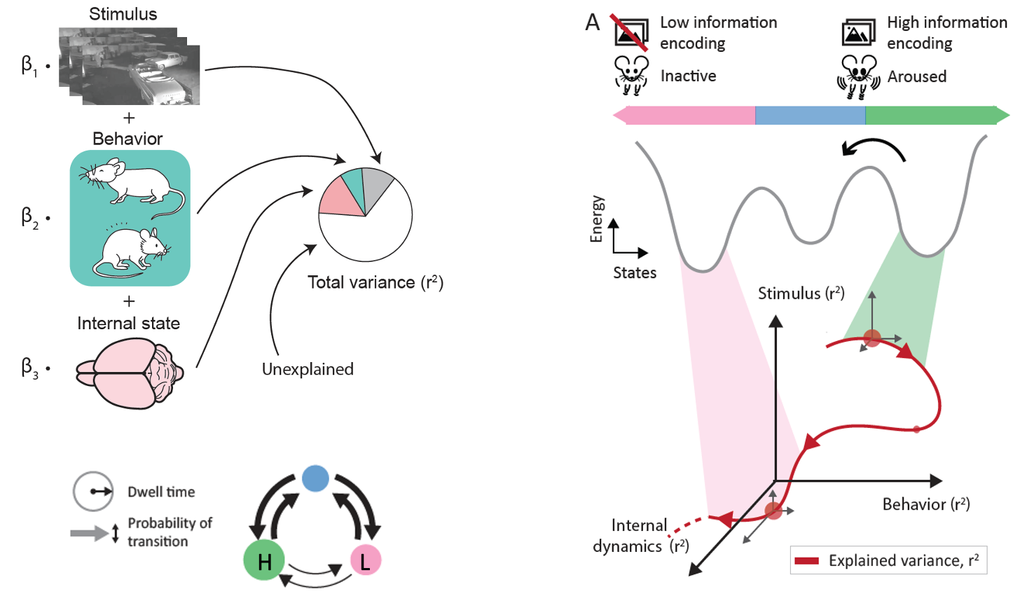
The scale of analysis made a striking difference. For individual neurons, visual stimulus features were the strongest predictors. For the average activity of whole visual areas, internal brain activity was the strongest predictor. Bodily movements contributed significantly at both scales, but during passive viewing of the natural movie they were rarely the dominant source.
These contributions also changed with state. Stimulus and behavioral features were most predictive in the high-frequency state. In the low-frequency state, adding LFPs and activity from neighboring areas produced a much larger improvement in prediction, indicating a stronger role for internal dynamics.
At the single-cell level, 53% of neurons in the low-frequency state belonged to a group for which no individual source explained more than 10% of their variance. When those same neurons entered the high-frequency state, about 40% shifted into a stimulus-dominated group. Neurons influenced by many sources also tended to become more specialized.
The dominant explanation for a neuron’s activity was therefore not a permanent label. It could change within seconds.
Encoding becomes more diverse along the hierarchy
The relative influence of different sources also depended on where a neuron was recorded.
Stimulus-dominated neurons were most common in V1 and became less common in higher visual areas. By contrast, neurons influenced by behavior or by multiple sources became more prevalent higher in the hierarchy. This suggests a gradual change from a population closely tied to visual input toward populations that integrate a broader mixture of sensory, behavioral, and internal signals.
That pattern does not mean higher areas stop representing the visual world. Rather, their responses appear to place visual information in a richer context—one that increasingly reflects what the animal is doing and the state of the wider brain.
Why conditioning on state changes the picture
If all trials are pooled together, a model returns an average of several different operating regimes. A factor that matters strongly in one state and weakly in another may appear only moderately important overall. Distinct cell populations may also look more homogeneous than they really are.
State conditioning makes those differences visible. It provides a way to ask not only what predicts a neural response? but also when does it predict that response?
This shift has practical implications. Comparisons across experiments, animals, cortical areas, or cell types can be misleading if the observations contain different mixtures of internal states. Models of sensory coding may become both more accurate and more interpretable when they explicitly account for non-stationarity.
What the study does—and does not—show
Several boundaries are important.
First, the study identifies statistical relationships, not causal mechanisms. Explained variance tells us how well a measured source predicts neural activity after the model’s controls; it does not prove that the source directly generates that activity.
Second, the three-state description is a useful and reproducible summary of LFP dynamics, but brain state may also vary continuously. Discrete states should be understood as an interpretable framework, not the only possible description of an awake brain.
Third, the mice passively viewed a natural movie. The balance among stimulus, behavior, and internal dynamics may differ during active perception, decision-making, or task engagement, and it may depend on the stimulus and recording method.
Finally, the association between the high-frequency state and stronger stimulus encoding does not by itself establish why the state improves encoding—or whether changing the state would causally change perception. Answering that question will require targeted perturbations alongside large-scale recording.
A neural code that changes with context
The visual cortex does not encode the world in isolation. Its responses emerge from an ongoing negotiation among external input, behavior, and internal dynamics.
Our results show that this negotiation is rapid. Within seconds, the brain can move into a different oscillation state, adopt a different variability profile, and redistribute which sources most strongly shape neural activity. The same movie can therefore meet a meaningfully different neural system from one moment to the next.
Understanding sensory coding requires more than asking what a neuron responds to on average. We also need to ask which state the brain is in when it responds.
Read the paper: Deciphering Neuronal Variability Across States Reveals Dynamic Sensory Encoding
Authors: Shailaja Akella, Peter Ledochowitsch, Joshua H. Siegle, Hannah Belski, Daniel D. Denman, Michael A. Buice, Severine Durand, Christof Koch, Shawn R. Olsen, and Xiaoxuan Jia.
Published in Nature Communications on February 19, 2025. The article is open access under a CC BY 4.0 license.